Depression detection based on speech data
Nadiia Novakova published on
22 min, 4234 words
Categories: Python Data Science Data Analysis Data Preparation
In this topic I would like to show how to manage a dataset with many features (especially numeric data with completely unclear meaning and influence on whole dataset)
The dataset contains speech features and clinical variables
from participants of a depression related study.
Based on speech recordings, vocal features have been derived from
different categories.
Each feature contains a tag _{pos,neg}, which refers to the vocal task it
was extracted from.
Clinical and demographic variables of participants can be found at the beginning.
The study was meant to show a relation between voice patterns and depression scale (variable ADS).
Description:
1: Participant identifier number in the study
2 - 4: Participant recorded demographic information
5: Depression score that records disturbances caused by depressive symptoms on a scale of 0-60. The participants can be classified into a group with (ADS > 17) and without (ADS < 17) depressive symptoms.
6 - 171: 84 speech features computed for negative and positive stories. Column names contain feature names and the story sentiment it was computed from. They are all separated by underscores i.e., speech_ratio_pos refers to speech ratio computed for positive stories.
172-215: 22 transcript features computed for negative and positive stories. Column names contain features name and the story sentiment it was computed, all separated by underscores i.e., adjective_rate_neg refers to adjective rate computed for negative stories.
import pandas as pd
from matplotlib import pyplot as plt
import os
import numpy as np
import seaborn as sns
from sklearn.preprocessing import LabelEncoder
from scipy.stats import  ttest_ind
import scipy.stats as stats
import warnings

warnings.filterwarnings('ignore')
df = pd.read_csv("data.csv")
df.shape
(121, 215)
Gender is a categorical variable. It should be transformed to numerical value:
df['gender'].unique()
array(['female', 'male'], dtype=object)
# Coding categorical feature "gender" as 0- male , 1- female
df_gender = df['gender'].map(lambda x:0 if x=='male' else 1)
df['gender'] = df_gender
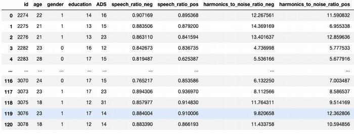
df.head()
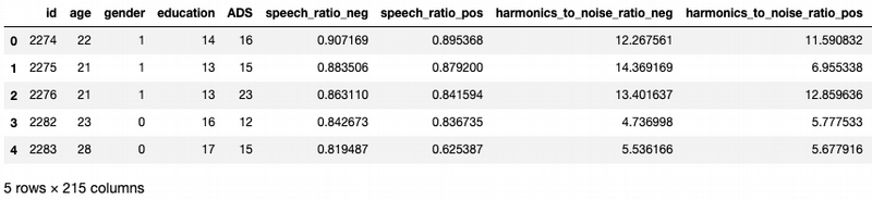
It is not enough data to divide data on to subsets by gender. So I will first explore and learn models with entire dataset. I will compare results afterwards. This dataset has 215 features. For more comfortable exploration I look at the feature cuts according the task description
df_demograph = df.iloc[:,:4]
df_sf = df.iloc[:,5:172]
df_tf = df.iloc[:,172:]
Previous data exploration shows that ADS can be a target variable. It is possible to classify participants as:
- 0 - "has depressive symptoms",
- 1 - "has no depressive symptoms"
df['ADS_cat']=df['ADS'].map(lambda x: 1 if x>17 else 0)
Data preparation
Let's explore all features with NaN or 0 values
def findNaNColumn (df):
    nan_columns = np.array([])
    for i in df.columns:
        if df[i].isnull().values.any():
            nan_columns = np.append(nan_columns, i)
    return nan_columns

a = findNaNColumn(df)
print(a)
['jitter_local_neg' 'jitter_absolute_neg' 'jitter_rap_neg'
'jitter_ppq5_neg' 'jitter_ddp_neg' 'jitter_local_pos'
'jitter_absolute_pos' 'jitter_rap_pos' 'jitter_ppq5_pos' 'jitter_ddp_pos']
def nan_amount(df,a):
for i in a:
    percent = str(round(df[i].isnull().sum()*100/df[i].count()))
    print(f"{i}: {percent}%")
# Amount of NaN data in columns
nan_amount(df,a)
jitter_local_neg: 9%
jitter_absolute_neg: 9%
jitter_rap_neg: 9%
jitter_ppq5_neg: 9%
jitter_ddp_neg: 9%
jitter_local_pos: 11%
jitter_absolute_pos: 11%
jitter_rap_pos: 11%
jitter_ppq5_pos: 11%
jitter_ddp_pos: 11%
NaN data here takes just near 10%, so it can be replaced by median values
def replaceNanOnMedian(a):
    for i in a:
        df[i] = df[i].fillna(df[i].median())

replaceNanOnMedian(a)
Columns with all zero values can be deleted
for i in df.columns:
    if df[i].mean() == 0.0:
        print(i+": "+str(df[i].mean()))
espinola_zero_crossing_metric_pos: 0.0
mean_number_subordinate_clauses_neg: 0.0
mean_number_subordinate_clauses_pos: 0.0
df =df.drop(['espinola_zero_crossing_metric_pos', \
    'mean_number_subordinate_clauses_neg', \
    'mean_number_subordinate_clauses_pos'], axis = 1)
Outliers influence elimination
For more accurate results feature sets should be normally distributed.
Demographical features
from scipy.stats import norm
sns.distplot(df['ADS'], fit = norm)
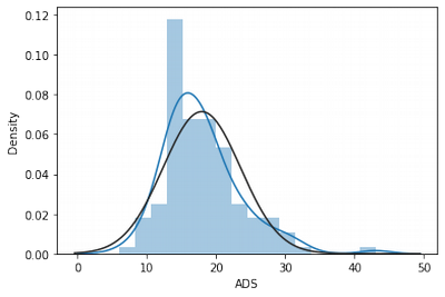
df['ADS'].skew()
1.2106132338523006
df['ADS'].kurtosis()
2.8349770036934183
sns.boxplot(df['ADS'])
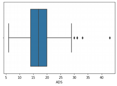
We can see that ADS has outliers, that is why it has right skew and quite big kurtosis
Let's try to normalise this feature set.
ADS Normality Exploration
#calculate lower and upper limit values for a sample

feature = 'ADS'
def boundary_values (feature):
    feature_q25,feature_q75 = np.percentile(df[feature], 25), np.percentile(df[feature], 75)
    feature_IQR = feature_q75 - feature_q25
    Threshold = feature_IQR * 1.5 #interquartile range (IQR)
    feature_lower, feature_upper = feature_q25 - Threshold, feature_q75 + Threshold
    print(f"Lower limit of {feature} distribution: {feature_lower}")
    print(f"Upper limit of {feature} distribution: {feature_upper}")
    return feature_lower,feature_upper;
#calculate limits
x,y = boundary_values(feature)
Lower limit of ADS distribution: 5.0
Upper limit of ADS distribution: 29.0
def manage_outliers(df,feature_lower,feature_upper):
    df_copy = df.copy()
    df_copy.loc[(df_copy[feature] > feature_upper),feature] = np.nan
    df_copy['ADS'].fillna(feature_upper, inplace=True)
    df_copy.loc[(df_copy[feature] < feature_lower),feature] = np.nan
    df_copy['ADS'].fillna(feature_lower, inplace=True)
    return df_copy;
df = manage_outliers(df,x,y)
df.agg(['skew', 'kurtosis']).transpose().loc['ADS']
skew        0.553851
kurtosis   -0.036457
Name: ADS, dtype: float64
sns.distplot(df['ADS'], fit = norm)
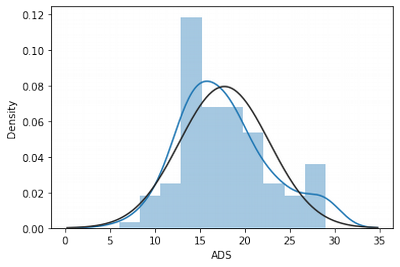
These transformations helped to decrease outlier influences as we see on the graph and by skew/kurtosis indexes.
Age Normality Exploration
sns.distplot(df['age'], fit = norm)
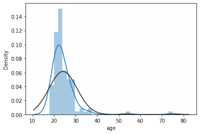
#calculate limits
feature='age'
x,y = boundary_values(feature)
Lower limit of age distribution: 13.5
Upper limit of age distribution: 33.5
n = df[df['age']>33.5]['age'].count()
print("Age outliers amount: "+str(n))
Age outliers amount: 5
print(str(n*100/df['age'].shape)+"%")
[4.1322314]%
Gender Normality Exploration
sns.displot(df['gender'])
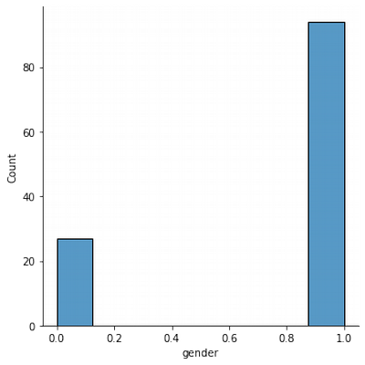
Women in test appear ~ 3 times more than men. It can influence the training quality further.
Education Normality Exploration
sns.distplot(df['education'], fit = norm)
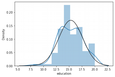
df.agg(['skew', 'kurtosis']).transpose().loc['education']
skew        0.007860
kurtosis   -0.137656
Name: education, dtype: float64
Education is more-less normally distributed. It can be fixed by standardisation on the next step.
Speech Features / Transcript Features Normality Exploration
df_sf= df.iloc[:,5:172]
df_sf
df_sf.shape[1]
167
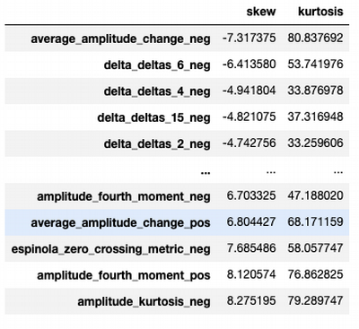
df_sf.agg(['skew', 'kurtosis']).transpose().loc[df_sf.columns].sort_values(by=['skew','kurtosis'])
def remove_zeros(dataframe):
    drop_cols = dataframe.columns[(dataframe == 0).sum() > 0.25 * dataframe.shape[1]]
    dataframe.drop(drop_cols, axis = 1, inplace = True)
    return dataframe
df_sf = remove_zeros(df_sf)
df_sf.shape
(121, 162)
df_tf= df.iloc[:,172:]
df_tf
df_tf = remove_zeros(df_tf)
df_sf.shape
(121, 162)
from scipy import stats
def shapiro_test(feature):
    p_value = stats.shapiro(df[feature])[0]
    print(f"{feature}: ")
    if p_value <=0.05:
        print("  distribution is non-normal")
    else:
        print("  distribution is normal")
for i in df_sf.columns:
    shapiro_test(i)
speech_ratio_neg:
distribution is normal
speech_ratio_pos:
distribution is normal
harmonics_to_noise_ratio_neg:
distribution is normal
...
...
...
distribution is normal
jitter_ppq5_pos:
distribution is normal
jitter_ddp_pos:
distribution is normal
for i in df_tf.columns:
    shapiro_test(i)
Both groups of features are normally distributed
Standardisation
from sklearn.preprocessing import StandardScaler
num_cols = df.iloc[:,3:df.shape[1]-1].columns
print(num_cols)
# apply standardisation on numerical features

for i in num_cols:
    scale = StandardScaler().fit(df[[i]])
    # transform the training data column
    df[i] = scale.transform(df[[i]])

scale = StandardScaler().fit(df[['age']])
df['age'] = scale.transform(df[['age']])
Index(['education', 'ADS', 'speech_ratio_neg', 'speech_ratio_pos',
'harmonics_to_noise_ratio_neg', 'harmonics_to_noise_ratio_pos',
'sound_to_noise_ratio_neg', 'sound_to_noise_ratio_pos', 'mean_f0_neg',
'mean_f0_pos',
...
'mean_cluster_density_neg', 'mean_cluster_density_pos',
'biggest_cluster_density_neg', 'biggest_cluster_density_pos',
'number_cluster_switches_neg', 'number_cluster_switches_pos',
'tangentiality_score_neg', 'tangentiality_score_pos',
'coherence_metric_neg', 'coherence_metric_pos'],
dtype='object', length=209)
df.drop('id',axis=1)
Modeling
Based on the type of target column we can see that we can apply binary classifiers. Logistic regression is obvious choice for that
Logistic regression
from sklearn.linear_model import LogisticRegression
from sklearn.metrics import classification_report, confusion_matrix
from sklearn.metrics import mean_squared_error
from sklearn.model_selection import train_test_split

X = df.copy()
X = X.drop('ADS_cat',axis=1)
X = X.drop('ADS',axis=1)
y = df['ADS_cat']

X_train, X_test, y_train, y_test = train_test_split(X,y,test_size=0.2,random_state=27)

model = LogisticRegression(solver='liblinear', random_state=0)
def train_test_model(model):
    model.fit(X_train, y_train)
    pred = model.predict(X_train)
    print(f"Predicted : {pred}")
    score = model.score(X_test, y_test)
    print(f"Score: {score}")
    return score
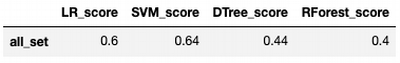
score = train_test_model(model)
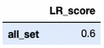
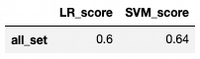
score_set = pd.DataFrame(data = [score], columns = ['LR_score'], index = ['all_set'])
Predicted : [1 0 0 1 1 1 0 0 0 0 1 0 1 1 0 0 1 0 0 1 0 0 0 1 0 0 0 0 0 1 0 0 0 0 1 0 1
0 0 0 1 0 1 0 0 1 0 1 0 0 0 0 0 0 0 1 1 1 1 0 0 1 1 1 1 1 0 0 0 1 0 0 0 1
1 1 0 1 0 1 0 1 0 0 1 1 1 0 1 1 0 0 1 0 1 1]
Score: 0.6
score_set
def conf_matrix(model, X_test, y_test):
cm = confusion_matrix(y_test, model.predict(X_test))
fig, ax = plt.subplots(figsize=(3, 3))
ax.imshow(cm)
ax.grid(False)
ax.xaxis.set(ticks=(0, 1), ticklabels=('Predicted 0s', 'Predicted 1s'))
ax.yaxis.set(ticks=(0, 1), ticklabels=('Actual 0s', 'Actual 1s'))
ax.set_ylim(1.5, -0.5)
for i in range(2):
for j in range(2):
ax.text(j, i, cm[i, j], ha='center', va='center', color='red')
plt.show()
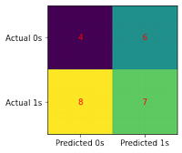
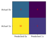
conf_matrix(model, X_test, y_test)
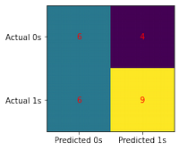
print(classification_report(y_test, model.predict(X_test)))

             precision    recall  f1-score   support

           0       0.50      0.60      0.55        10
           1       0.69      0.60      0.64        15

    accuracy                           0.60        25
   macro avg       0.60      0.60      0.59        25
weighted avg       0.62      0.60      0.60        25
Accuracy value is not good enough. Let's try other binary classifiers.
Support vector machine
from sklearn import svm
model = svm.SVC(kernel='linear', C=1,gamma='auto')
score_set['SVM_score'] = train_test_model(model)
Predicted : [1 0 0 1 1 1 0 0 0 0 1 0 1 1 0 0 1 0 0 1 0 0 0 1 0 0 0 0 0 1 0 0 0 0 1 0 1
0 0 0 1 0 1 0 0 1 0 1 0 0 0 0 0 0 0 1 1 1 1 0 0 1 1 1 1 1 0 0 0 1 0 0 0 1
1 1 0 1 0 1 0 1 0 0 1 1 1 0 1 1 0 0 1 0 1 1]
Score: 0.64
conf_matrix(model, X_test, y_test)
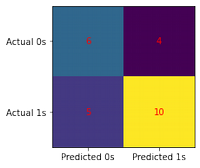
print(classification_report(y_test, model.predict(X_test)))
              precision    recall  f1-score   support

           0       0.55      0.60      0.57        10
           1       0.71      0.67      0.69        15

    accuracy                           0.64        25
   macro avg       0.63      0.63      0.63        25
weighted avg       0.65      0.64      0.64        25
score_set
Decission Tree
from sklearn.tree import DecisionTreeClassifier
from sklearn import metrics
# Create Decision Tree classifier object
model = DecisionTreeClassifier()
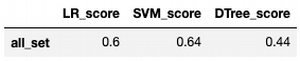
score_set['DTree_score'] = train_test_model(model)
Predicted : [1 0 0 1 1 1 0 0 0 0 1 0 1 1 0 0 1 0 0 1 0 0 0 1 0 0 0 0 0 1 0 0 0 0 1 0 1
0 0 0 1 0 1 0 0 1 0 1 0 0 0 0 0 0 0 1 1 1 1 0 0 1 1 1 1 1 0 0 0 1 0 0 0 1
1 1 0 1 0 1 0 1 0 0 1 1 1 0 1 1 0 0 1 0 1 1]
Score: 0.44
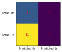
conf_matrix(model, X_test, y_test)
print(classification_report(y_test, model.predict(X_test)))
             precision    recall  f1-score   support

           0       0.33      0.40      0.36        10
           1       0.54      0.47      0.50        15

    accuracy                           0.44        25
   macro avg       0.44      0.43      0.43        25
weighted avg       0.46      0.44      0.45        25
score_set
Random Forest
from sklearn.ensemble import RandomForestClassifier
# Instantiate model with 100 decision trees
model = RandomForestClassifier(n_estimators=100)

score_set['RForest_score'] = train_test_model(model)
Predicted : [1 0 0 1 1 1 0 0 0 0 1 0 1 1 0 0 1 0 0 1 0 0 0 1 0 0 0 0 0 1 0 0 0 0 1 0 1
0 0 0 1 0 1 0 0 1 0 1 0 0 0 0 0 0 0 1 1 1 1 0 0 1 1 1 1 1 0 0 0 1 0 0 0 1
1 1 0 1 0 1 0 1 0 0 1 1 1 0 1 1 0 0 1 0 1 1]
Score: 0.4
conf_matrix(model, X_test, y_test)
print(classification_report(y_test, model.predict(X_test)))
             precision    recall  f1-score   support

           0       0.35      0.60      0.44        10
           1       0.50      0.27      0.35        15

    accuracy                           0.40        25
   macro avg       0.43      0.43      0.40        25
weighted avg       0.44      0.40      0.39        25
score_set
Naive Bayes
from sklearn.naive_bayes import GaussianNB
#Create a Gaussian Classifier
model = GaussianNB()
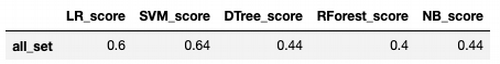
score_set['NB_score'] = train_test_model(model)
Predicted : [1 0 0 1 0 1 0 0 0 0 0 1 0 1 0 0 1 0 0 1 0 0 0 1 0 0 0 0 0 0 1 0 0 0 1 1 1
0 0 0 1 0 0 0 0 0 0 0 0 0 0 0 0 0 0 0 1 1 1 0 0 1 1 0 1 1 0 0 0 1 0 0 0 0
0 1 0 1 0 0 0 1 0 1 1 0 0 0 0 1 0 0 0 0 1 0]
Score: 0.44
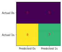
conf_matrix(model, X_test, y_test)
print(classification_report(y_test, model.predict(X_test)))
score_set
KNN
from sklearn.neighbors import KNeighborsClassifier

model = KNeighborsClassifier(n_neighbors=3)
score_set['KNN_score'] = train_test_model(model)
Predicted : [1 0 0 1 1 1 0 0 0 1 1 1 1 1 0 0 1 1 0 1 0 0 1 1 1 0 0 1 0 1 0 0 0 1 1 0 1
0 0 0 1 1 1 1 0 1 0 1 0 0 0 1 0 0 0 1 1 0 1 0 0 1 1 0 0 0 0 0 0 1 1 0 1 1
1 0 0 1 0 1 0 1 0 1 1 0 1 0 0 1 0 0 1 0 0 1]
Score: 0.48
conf_matrix(model, X_test, y_test)
print(classification_report(y_test, model.predict(X_test)))
             precision    recall  f1-score   support

           0       0.38      0.50      0.43        10
           1       0.58      0.47      0.52        15

    accuracy                           0.48        25
   macro avg       0.48      0.48      0.48        25
weighted avg       0.50      0.48      0.49        25
score_set
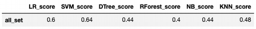
Logistic Regression and SVM got the best results, but not enough good.
Correlation exploration
To increase model scores, it make sense to decrease amount of features. For that, we need to find more correlated ones with ADS.
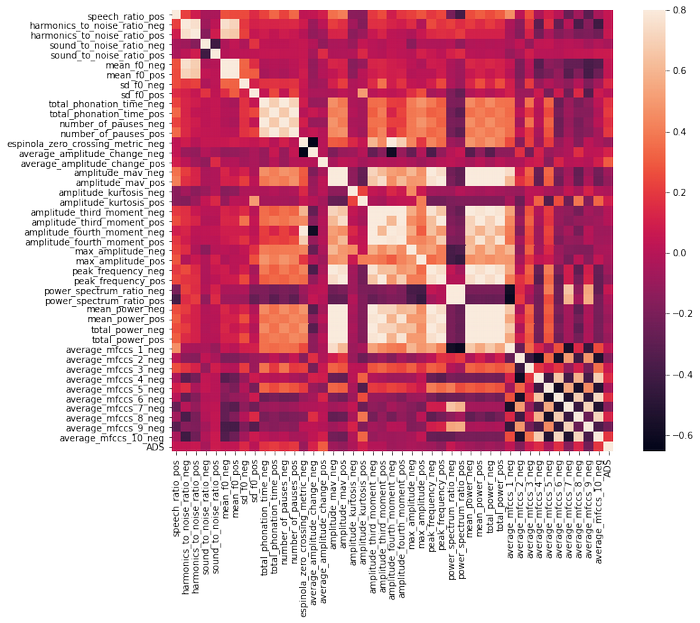
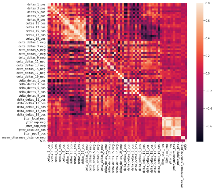
It is too many features to visualise correlation, so I am dividing them into chunks:
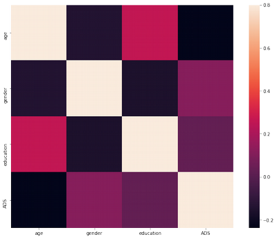
#correlation matrix
df_demograph = df.iloc[:,1:5]
corrmat = df_demograph.corr()
f, ax = plt.subplots(figsize=(12, 9))
sns.heatmap(corrmat, vmax=.8, square=True);
#correlation matrix
df_sf= df.iloc[:,6:50]
df_sf['ADS'] = df['ADS']
corrmat = df_sf.corr()
f, ax = plt.subplots(figsize=(12, 9))
sns.heatmap(corrmat, vmax=.8, square=True);
df_sf= df.iloc[:,50:100]
df_sf['ADS'] = df['ADS']
corrmat = df_sf.corr()
f, ax = plt.subplots(figsize=(12, 9))
sns.heatmap(corrmat, vmax=.8, square=True);
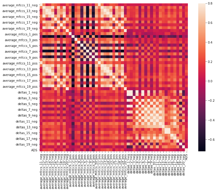
df_sf= df.iloc[:,100:172]
df_sf['ADS'] = df['ADS']
corrmat = df_sf.corr()
f, ax = plt.subplots(figsize=(12, 9))
sns.heatmap(corrmat, vmax=.8, square=True);
df_tf= df.iloc[:,172:]
df_tf['ADS'] = df['ADS']
corrmat = df_sf.corr()
f, ax = plt.subplots(figsize=(12, 9))
sns.heatmap(corrmat, vmax=.8, square=True);

There is no strong correlation between ADS and other features.
Extract all features which have at least absolute correlation > 0.2:
short_df = df.copy()
short_df = short_df.drop(['id'],axis=1)
corrmat = short_df.corr()

new_feature_set = corrmat[abs(corrmat['ADS']>=0.2)].index
print("New feature set indeses: ")
print(new_feature_set)
selected_columns = short_df[new_feature_set]

short_df = selected_columns.copy()

short_df = short_df.drop('ADS',axis = 1)
New feature set indexes:
Index(['ADS', 'total_phonation_time_pos', 'average_amplitude_change_pos',
'average_mfccs_12_neg', 'average_mfccs_14_neg', 'average_mfccs_15_neg',
'average_mfccs_19_neg', 'average_mfccs_12_pos', 'average_mfccs_13_pos',
'average_mfccs_14_pos', 'average_mfccs_15_pos', 'delta_deltas_7_pos',
'delta_deltas_9_pos', 'verb_rate_pos', 'avg_dep_distance_neg',
'total_dep_distance_neg', 'avg_dependencies_neg',
'avg_dependencies_pos', 'mean_cluster_size_neg',
'mean_cluster_density_neg', 'mean_cluster_density_pos',
'biggest_cluster_density_neg', 'biggest_cluster_density_pos',
'ADS_cat'],
dtype='object')
short_df['age'] = df['age']
short_df['gender'] = df['gender']
short_df['education'] = df['education']
Trying to train/validate model with less features for LR and SVM for the first approach:
X = short_df.copy()
X = X.drop('ADS_cat',axis=1)
y = short_df['ADS_cat']

X_train, X_test, y_train, y_test = train_test_split(X,y,test_size=0.2,random_state=27)

model = LogisticRegression(solver='liblinear', random_state=0)
score = train_test_model(model)
Predicted : [1 0 1 0 1 1 0 0 0 0 1 0 0 1 0 0 1 0 0 0 0 0 0 1 1 1 0 0 0 0 0 0 1 0 1 1 0
0 0 0 1 0 0 0 0 0 1 1 0 0 0 0 1 1 0 0 1 1 1 0 0 1 1 0 1 0 0 0 0 1 0 0 0 0
1 0 0 1 0 1 0 1 0 1 1 0 1 0 0 1 0 0 0 0 1 0]
Score: 0.48
model = svm.SVC(kernel='linear', C=1,gamma='auto')
score_set['SVM_score'] = train_test_model(model)
Predicted : [1 0 1 0 1 1 0 0 0 0 1 0 0 1 0 0 1 0 0 0 0 0 0 1 0 1 0 0 0 0 0 0 0 0 1 1 1
0 0 0 1 0 0 0 0 0 0 1 1 0 0 0 1 1 0 0 1 1 1 0 0 1 1 0 1 0 0 0 0 1 0 0 0 0
1 0 0 1 0 1 0 1 0 1 1 0 1 0 0 1 0 0 0 0 1 0]
Score: 0.52
Accuracy of algorithms reduced due to decreasing number of features.
Exploration by Gender
Divide data by gender
df_male = df[df['gender']=='male']
df.drop(['gender'], axis = 1)
df_female = df[df['gender']=='female']
df.drop(['gender'], axis = 1)

df_male.shape
(0, 213)
df_female.shape
(0, 213)
df_male = df.loc[df['gender']==0]
df_male = df_male.drop('gender',axis=1)
df_female = df.loc[df['gender']==1]
df_female = df_female.drop('gender',axis=1)
df_female
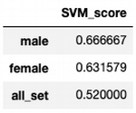
Let's try the male/female datasets for two algorithms with the best accuracy for the whole dataset: SVM and Logistic Regression
X = df_male.copy()
X = X.drop('ADS_cat',axis=1)
X = X.drop('ADS',axis=1)
y = df_male['ADS_cat']

X_train, X_test, y_train, y_test = train_test_split(X,y,test_size=0.2,random_state=27)
model = LogisticRegression(solver='liblinear', random_state=0)
score = train_test_model(model)
gender_score_set =  pd.DataFrame(data = [score] ,columns =['LR_score'], index = ['male'])

X = df_female.copy()
X = X.drop('ADS_cat',axis=1)
X = X.drop('ADS',axis=1)
y = df_female['ADS_cat']

X_train, X_test, y_train, y_test = train_test_split(X,y,test_size=0.2,random_state=27)
model = LogisticRegression(solver='liblinear', random_state=0)
gender_score_set.loc['female']  = train_test_model(model)

gender_score_set.loc['all_set']  = score_set['LR_score'].loc['all_set']
Predicted : [1 1 0 0 1 0 0 0 0 0 1 0 0 0 1 0 1 0 1 1 0]
Score: 0.6666666666666666
Predicted : [0 1 1 0 1 0 1 1 0 1 0 0 0 1 1 0 0 0 1 1 0 1 1 0 0 1 0 0 1 1 1 0 1 1 0 0 1
1 0 0 0 0 0 1 0 1 1 0 0 0 1 0 1 1 0 1 1 0 1 0 1 1 0 1 0 1 0 1 0 1 0 0 1 0
0]
Score: 0.5263157894736842
gender_score_set
X = df_male.copy()
X = X.drop('ADS_cat',axis=1)
X = X.drop('ADS',axis=1)
y = df_male['ADS_cat']

X_train, X_test, y_train, y_test = train_test_split(X,y,test_size=0.2,random_state=27)

model = svm.SVC(kernel='linear', C=1,gamma='auto')

score = train_test_model(model)
gender_score_set =  pd.DataFrame(data = [score] ,columns =['SVM_score'], index = ['male'])

X = df_female.copy()
X = X.drop('ADS_cat',axis=1)
X = X.drop('ADS',axis=1)
y = df_female['ADS_cat']

X_train, X_test, y_train, y_test = train_test_split(X,y,test_size=0.2,random_state=27)
model = svm.SVC(kernel='linear', C=1,gamma='auto')
gender_score_set.loc['female']  = train_test_model(model)

gender_score_set.loc['all_set']  = score_set['SVM_score'].loc['all_set']
Predicted : [1 1 0 0 1 0 0 0 0 0 1 0 0 0 1 0 1 0 1 1 0]
Score: 0.6666666666666666
Predicted : [0 1 1 0 1 0 1 1 0 1 0 0 0 1 1 0 0 0 1 1 0 1 1 0 0 1 0 0 1 1 1 0 1 1 0 0 1
1 0 0 0 0 0 1 0 1 1 0 0 0 1 0 1 1 0 1 1 0 1 0 1 1 0 1 0 1 0 1 0 1 0 0 1 0
0]
Score: 0.631578947368421
gender_score_set
Dividing on subsets gives higher classification accuracy just in male gender group, and lower for female.
Cross Validation as classification improvement approach
Cross validation may help to improve training.
Initial Set
from sklearn.model_selection import cross_val_score, cross_val_predict

def scoring(df):
    X = df.copy()
    X = X.drop('ADS_cat',axis=1)
    X = X.drop('ADS',axis=1)
    y = df['ADS_cat']
    #----------------------------------------------------------------
    model = LogisticRegression(solver='liblinear', random_state=0)
    scores = cross_val_score(model, df, y, cv=5)
    print("Logistic Regression: ")
    print(f"Score: {scores}")
    print("The best fold score: ", scores.max())

    score_set_cv = pd.DataFrame(data = [scores.max()] ,columns =['LR_score'], index = ['all_set_CV'])
    #----------------------------------------------------------------
    model = svm.SVC(kernel='linear',C=1,gamma='auto')
    scores = cross_val_score(model, df, y, cv=5)
    print("SVM: ")
    print(f"Score: {scores}")
    print("The best fold score: ", scores.max())

    score_set_cv['SVM_score']=scores.max()
    #----------------------------------------------------------------
    model = DecisionTreeClassifier()
    scores = cross_val_score(model, df, y, cv=5)
    print("DTree: ")
    print(f"Score: {scores}")
    print("The best fold score: ", scores.max())

    score_set_cv['DTree_score']=scores.max()
    #----------------------------------------------------------------
    model = RandomForestClassifier(n_estimators=100)
    scores = cross_val_score(model, df, y, cv=5)
    print("RForest: ")
    print(f"Score: {scores}")
    print("The best fold score: ", scores.max())

    score_set_cv['RForest_score']=scores.max()
    #----------------------------------------------------------------
    model = GaussianNB()
    scores = cross_val_score(model, df, y, cv=5)
    print("Naive Bayes: ")
    print(f"Score: {scores}")
    print("The best fold score: ", scores.max())

    score_set_cv['NB_score']=scores.max()
    #----------------------------------------------------------------
    model = KNeighborsClassifier(n_neighbors=3)
    scores = cross_val_score(model, df, y, cv=5)
    print("KNN: ")
    print(f"Score: {scores}")
    print("The best fold score: ", scores.max())

    score_set_cv['KNN_score']=scores.max()
    return score_set_cv
    #----------------------------------------------------------------

score = scoring(df)
print(score)
Logistic Regression:
Score: [0.92 0.83333333 0.91666667 0.83333333 0.91666667]
The best fold score: 0.92
SVM:
Score: [0.92 0.91666667 0.875 0.83333333 0.875 ]
The best fold score: 0.92
DTree:
Score: [1. 1. 1. 1. 1.]
The best fold score: 1.0
RForest:
Score: [0.96 0.95833333 1. 1. 1. ]
The best fold score: 1.0
Naive Bayes:
Score: [1. 1. 0.95833333 1. 1. ]
The best fold score: 1.0
KNN:
Score: [0.52 0.45833333 0.33333333 0.625 0.45833333]
The best fold score: 0.625
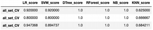
LR_score SVM_score DTree_score RForest_score NB_score \
all_set_CV 0.92 0.92 1.0 1.0 1.0
KNN_score
all_set_CV 0.625
For Male/Female Subsets
score_set_cv_male = scoring(df_male)
print(score_set_cv_male)
Logistic Regression:
Score: [0.66666667 0.66666667 0.4        0.8        0.8       ]
The best fold score:  0.8
SVM:
Score: [0.66666667 0.66666667 0.6        0.8        0.6       ]
The best fold score:  0.8
DTree:
Score: [1. 1. 1. 1. 1.]
The best fold score:  1.0
RForest:
Score: [0.66666667 0.66666667 0.8        1.         1.        ]
The best fold score:  1.0
Naive Bayes:
Score: [1.  1.  0.8 1.  1. ]
The best fold score:  1.0
KNN:
Score: [0.66666667 0.5        0.4        0.2        0.6       ]
The best fold score:  0.6666666666666666
LR_score  SVM_score  DTree_score  RForest_score  NB_score  \
all_set_CV       0.8        0.8          1.0            1.0       1.0

            KNN_score
all_set_CV   0.666667
score_set_cv_female = scoring(df_female)
print(score_set_cv_female)
Logistic Regression:
Score: [0.94736842 0.68421053 0.94736842 0.89473684 0.94444444]
The best fold score:  0.9473684210526315
SVM:
Score: [0.89473684 0.68421053 0.84210526 0.84210526 0.83333333]
The best fold score:  0.8947368421052632
DTree:
Score: [1. 1. 1. 1. 1.]
The best fold score:  1.0
RForest:
Score: [1.         0.78947368 1.         1.         0.88888889]
The best fold score:  1.0
Naive Bayes:
Score: [1. 1. 1. 1. 1.]
The best fold score:  1.0
KNN:
Score: [0.47368421 0.31578947 0.26315789 0.68421053 0.5       ]
The best fold score:  0.6842105263157895
LR_score  SVM_score  DTree_score  RForest_score  NB_score  \
all_set_CV  0.947368   0.894737          1.0            1.0       1.0

            KNN_score
all_set_CV   0.684211
RESULTS
result = pd.concat([score_set_cv , score_set_cv_male, score_set_cv_female])
Summary
- Logistic regression gives the best results on all subsets after cross-validation.
- SVM has very close (good) results.
- Decision Tree, Random Forest, Naive Bayes look like overfitting.
- KNN is not good enough comparing to the first a couple of models.
- There is a probability that overall modelling results would be better, if having bigger dataset.