Basic Feature Engineering Techniques for ML
In this topic I want to describe some basic data transformation and analysing techniques to prepare data for modelling. For demonstration I took Medical Cost Personal Datasets from Kaggle.
Medical Cost Personal Datasets Insurance Forecast by using Linear Regression
import pandas as pd
from matplotlib import pyplot as plt
import os
import numpy as np
import seaborn as sns
from sklearn.preprocessing import LabelEncoder
from scipy.stats import  ttest_ind
import scipy.stats as stats
import warnings
warnings.filterwarnings('ignore')
os.chdir('/python/insurence/')
df = pd.read_csv("insurance.csv")
df.head(5)
| age | sex | bmi | children | smoker | region | charges | |
|---|---|---|---|---|---|---|---|
| 0 | 19 | female | 27.900 | 0 | yes | southwest | 16884.92400 |
| 1 | 18 | male | 33.770 | 1 | no | southeast | 1725.55230 |
| 2 | 28 | male | 33.000 | 3 | no | southeast | 4449.46200 |
| 3 | 33 | male | 22.705 | 0 | no | northwest | 21984.47061 |
| 4 | 32 | male | 28.880 | 0 | no | northwest | 3866.85520 |
Numerical
-
age: age of primary beneficiary
-
bmi: body mass index, providing an understanding of a body, weights that are relatively high or low relative to height, objective index of body weight (kg / m ^ 2) using the ratio of height to weight, ideally 18.5 to 24.9
-
charges: individual medical costs billed by health insurance
-
children: number of children covered by health insurance / number of dependents
Categorical
-
sex: insurance contractor gender, female, male
-
smoker: smoking or not
-
region: the beneficiary's residential area in the US, northeast, southeast, southwest, northwest.
df.describe()
| age | bmi | children | charges | |
|---|---|---|---|---|
| count | 1338.000000 | 1338.000000 | 1338.000000 | 1338.000000 |
| mean | 39.207025 | 30.663397 | 1.094918 | 13270.422265 |
| std | 14.049960 | 6.098187 | 1.205493 | 12110.011237 |
| min | 18.000000 | 15.960000 | 0.000000 | 1121.873900 |
| 25% | 27.000000 | 26.296250 | 0.000000 | 4740.287150 |
| 50% | 39.000000 | 30.400000 | 1.000000 | 9382.033000 |
| 75% | 51.000000 | 34.693750 | 2.000000 | 16639.912515 |
| max | 64.000000 | 53.130000 | 5.000000 | 63770.428010 |
df.info()


<class 'pandas.core.frame.DataFrame'>
RangeIndex: 1338 entries, 0 to 1337
Data columns (total 7 columns):
  #   Column    Non-Null Count  Dtype
---  ------    --------------  -----
  0   age       1338 non-null   int64
  1   sex       1338 non-null   object
  2   bmi       1338 non-null   float64
  3   children  1338 non-null   int64
  4   smoker    1338 non-null   object
  5   region    1338 non-null   object
  6   charges   1338 non-null   float64
dtypes: float64(2), int64(2), object(3)
memory usage: 73.3+ KB
Charges distribution
Let's research the distributions for numerical features of the set. Start with charges and analyse its distribution. Our goal is to make normal distribution for each feature before starting using this data in modelling.
#Charges distribution
sns.distplot(df['charges'])
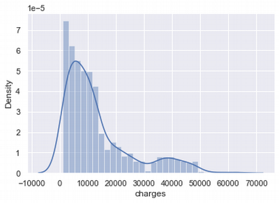
We can see that charges normal distribution is asymmetrical.
Task of the data scientist during the feature preparation is to achieve data uniformity.
There are some techniques for that to apply see more here or here.
- Imputation
- Handling Outliers
- Binning
- Log Transform
- Feature Encoding
- Grouping Operations
- Scaling
We will apply some of them depends on what behaviour we will have in feature samples.
Outliers in charges
Let's check how much outliers in charges distribution.
sns.boxplot(x=df['charges'])
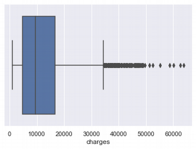
There are a lot of outliers from the right side. Tere are some imputation approaches for that. I'll try to delete outliers or replace outliers by median value and compare results.
#Set feature
feature = 'charges'
Imputation and Handling outliers
Below I am calculating limit the lower and upper values for a sample. Values outside of this range (lover limit, upper limit) are outliers.
#calculate lower and upper limit values for a sample
def boundary_values (feature):
    feature_q25,feature_q75 = np.percentile(df[feature], 25), np.percentile(df[feature], 75)
    feature_IQR = feature_q75 - feature_q25
    Threshold = feature_IQR * 1.5 #interquartile range (IQR)
    feature_lower, feature_upper = feature_q25-Threshold, feature_q75 + Threshold
    print("Lower limit of " + feature + " distribution: " + str(feature_lower))
    print("Upper limit of " + feature + " distribution: " + str(feature_upper))
    return feature_lower,feature_upper;


#create two new DF with transformed/deleted outliers
#1st - outliers changed on sample median
#2nd - deleting outliers
def manage_outliers(df,feature_lower,feature_upper):
    df_del = df.copy()
    df_median = df.copy()

    median = df_del.loc[(df_del[feature] < feature_upper) & \
      (df_del[feature] > feature_lower), feature].median()

    df_del.loc[(df_del[feature] > feature_upper)] = np.nan
    df_del.loc[(df_del[feature] < feature_lower)] = np.nan

    df_del.fillna(median, inplace=True)

    df_median.loc[(df_median[feature] > charges_upper)] = np.nan
    df_median.loc[(df_median[feature] < charges_lower)] = np.nan
    df_median.dropna(subset = [feature], inplace=True)

    return df_del, df_median;
#calculate limits
x,y = boundary_values(feature)

#samples with modified outliers
df_median, df_del = manage_outliers(df,x,y)
Lower limit of charges distribution: -13109.1508975
Upper limit of charges distribution: 34489.350562499996
df_median['charges'].mean()
9770.084335798923
df_agg = pd.DataFrame(
    {'df': [
        df['charges'].mean(),
        df['charges'].max(),
        df['charges'].min(),
        df['charges'].std(),
        df['charges'].count()]
     }, columns=['df'], index=['mean', 'max', 'min', 'std', 'count'])

df_agg['df_mean'] = pd.DataFrame(
    {'df_median': [
        df_median['charges'].mean(),
        df_median['charges'].max(),
        df_median['charges'].min(),
        df_median['charges'].std(),
        df_median['charges'].count()]
     }, columns=['df_median'], index=['mean', 'max', 'min', 'std', 'count'])

df_agg['df_del'] = pd.DataFrame(
    {'df_del': [
        df_del['charges'].mean(),
        df_del['charges'].max(),
        df_del['charges'].min(),
        df_del['charges'].std(),
        df_del['charges'].count()]
     }, columns=['df_del'], index=['mean', 'max', 'min', 'std', 'count'])

df_agg
| df | df_mean | df_del | |
|---|---|---|---|
| mean | 13270.422265 | 9770.084336 | 9927.753402 |
| max | 63770.428010 | 34472.841000 | 34472.841000 |
| min | 1121.873900 | 1121.873900 | 1121.873900 |
| std | 12110.011237 | 6870.056585 | 7241.158309 |
| count | 1338.000000 | 1338.000000 | 1199.000000 |
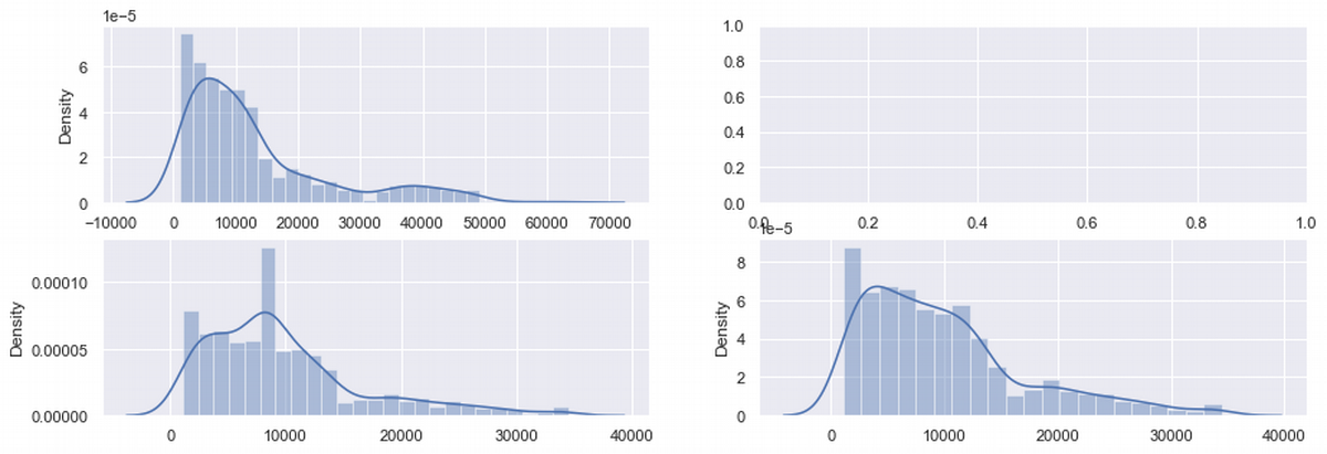
#the sample after sample modification

fig, ax = plt.subplots(2,2, figsize=(15, 5))

sns.distplot(ax = ax[0,0], x = df['charges'])
sns.distplot(ax = ax[1,0], x = df_median['charges'])
sns.distplot(ax = ax[1,1], x = df_del['charges'])
plt.show()
df_shape = df.agg(['skew', 'kurtosis']).transpose()
df_shape.rename(columns = {'skew':'skew_df','kurtosis':'kurtosis_df'}, inplace = True)
df_shape['skew_median'] = df_median.agg(['skew', 'kurtosis']).transpose()['skew']
df_shape['kurtosis_median'] = df_median.agg(['skew', 'kurtosis']).transpose()['kurtosis']
df_shape['skew_del'] = df_del.agg(['skew', 'kurtosis']).transpose()['skew']
df_shape['kurtosis_del'] = df_del.agg(['skew', 'kurtosis']).transpose()['kurtosis']
df_shape
| skew_df | kurtosis_df | skew_median | kurtosis_median | skew_del | kurtosis_del | |
|---|---|---|---|---|---|---|
| age | 0.055673 | -1.245088 | 2.599285 | 4.763691 | 0.067588 | -1.255101 |
| bmi | 0.284047 | -0.050732 | 2.599394 | 4.764021 | 0.366750 | 0.011529 |
| children | 0.938380 | 0.202454 | 2.599417 | 4.764092 | 0.987108 | 0.318218 |
| charges | 1.515880 | 1.606299 | 1.304122 | 1.565420 | 1.178483 | 1.022970 |
Let's look at the charges row. Here is some positive changes: skew and kurtosis decreased, but still not significantly. So charges still need additional improvements.
There are a few data transformation methods solving abnormality. We will try two of them (Square Root and Log) and choose better for the dataset.
Square Root transformation
Square root method is typically used when your data is moderately skewed, see more here.
df.insert(len(df.columns), 'charges_Sqrt',np.sqrt(df.iloc[:,6]))
df_median.insert(len(df_median.columns), 'charges_Sqrt',np.sqrt(df_median.iloc[:,6]))
df_del.insert(len(df_del.columns), 'charges_Sqrt',np.sqrt(df_del.iloc[:,6]))
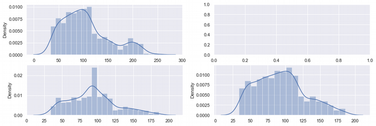
fig, ax = plt.subplots(2,2, figsize=(15, 5))

sns.distplot(ax = ax[0,0], x = df['charges_Sqrt'])
sns.distplot(ax = ax[1,0], x = df_median['charges_Sqrt'])
sns.distplot(ax = ax[1,1], x = df_del['charges_Sqrt'])
plt.show()
df_shape_sqrt = df.agg(['skew', 'kurtosis']).transpose()
df_shape_sqrt.rename(columns = {'skew':'skew_df','kurtosis':'kurtosis_df'}, inplace = True)
df_shape_sqrt['skew_median'] = df_median.agg(['skew', 'kurtosis']).transpose()['skew']
df_shape_sqrt['kurtosis_median'] = df_median.agg(['skew', 'kurtosis']).transpose()['kurtosis']
df_shape_sqrt['skew_del'] = df_del.agg(['skew', 'kurtosis']).transpose()['skew']
df_shape_sqrt['kurtosis_del'] = df_del.agg(['skew', 'kurtosis']).transpose()['kurtosis']
df_shape_sqrt
| skew_df | kurtosis_df | skew_median | kurtosis_median | skew_del | kurtosis_del | |
|---|---|---|---|---|---|---|
| age | 0.055673 | -1.245088 | 2.599285 | 4.763691 | 0.067588 | -1.255101 |
| bmi | 0.284047 | -0.050732 | 2.599394 | 4.764021 | 0.366750 | 0.011529 |
| children | 0.938380 | 0.202454 | 2.599417 | 4.764092 | 0.987108 | 0.318218 |
| charges | 1.515880 | 1.606299 | 1.304122 | 1.565420 | 1.178483 | 1.022970 |
| charges_Sqrt | 0.795863 | -0.073061 | 0.479111 | -0.089718 | 0.440043 | -0.399537 |
Log transformation
# Python log transform
df.insert(len(df.columns), 'charges_log',np.log(df['charges']))
df_median.insert(len(df_median.columns), 'charges_log',np.log(df_median['charges']))
df_del.insert(len(df_del.columns), 'charges_log',np.log(df_del['charges']))
df_shape_log = df.agg(['skew', 'kurtosis']).transpose()
df_shape_log.rename(columns = {'skew':'skew_df','kurtosis':'kurtosis_df'}, inplace = True)
df_shape_log['skew_median'] = df_median.agg(['skew', 'kurtosis']).transpose()['skew']
df_shape_log['kurtosis_median'] = df_median.agg(['skew', 'kurtosis']).transpose()['kurtosis']
df_shape_log['skew_del'] = df_del.agg(['skew', 'kurtosis']).transpose()['skew']
df_shape_log['kurtosis_del'] = df_del.agg(['skew', 'kurtosis']).transpose()['kurtosis']
df_shape_log
| skew_df | kurtosis_df | skew_median | kurtosis_median | skew_del | kurtosis_del | |
|---|---|---|---|---|---|---|
| age | 0.055673 | -1.245088 | 2.599285 | 4.763691 | 0.067588 | -1.255101 |
| bmi | 0.284047 | -0.050732 | 2.599394 | 4.764021 | 0.366750 | 0.011529 |
| children | 0.938380 | 0.202454 | 2.599417 | 4.764092 | 0.987108 | 0.318218 |
| charges | 1.515880 | 1.606299 | 1.304122 | 1.565420 | 1.178483 | 1.022970 |
| charges_Sqrt | 0.795863 | -0.073061 | 0.479111 | -0.089718 | 0.440043 | -0.399537 |
| charges_log | -0.090098 | -0.636667 | -0.393856 | -0.319703 | -0.328473 | -0.609327 |
fig, ax = plt.subplots(2,2, figsize=(15, 5))

sns.distplot(ax = ax[0,0], x = df['charges_log'])
sns.distplot(ax = ax[1,0], x = df_median['charges_log'])
sns.distplot(ax = ax[1,1], x= df_del['charges_log'])
plt.show()
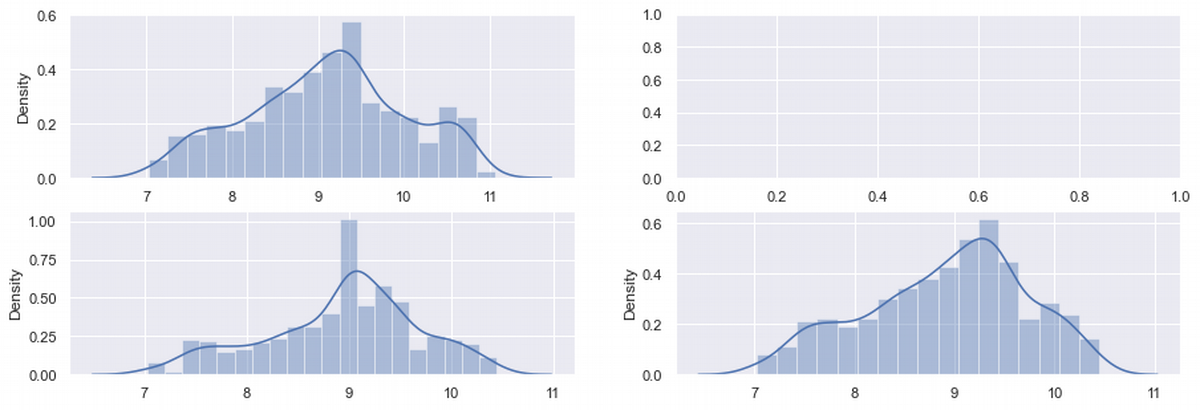
Here in table we can compare pairs skew-kurtosis for three DF: unmodified, with outliers changed on mean and with deleted outliers.
The first three pare for charges DF looks non-normal, because both in pair are enough far from 0.
After Square-Root transformations the best pair is a mediand_df pair with lower skew and kurtosis in the same time.
If compare with Log-transformation, the best values for normal distribution is in the initial DF.
For df_del there are a good result in solving skewness issue.
Log-transformation works good with asymmetrical data.
If we compare shapes on the graphs, we see there that initial DF is more symmetrical.
Interim conclusions: Distribution is still non-normal. But anyway the previous transformations get us some enough good results and allow to work with data further. For a modelling it makes sense to use log-transformed charges or square-root-transformed charges and outliers replaced by medians. Deleting outliers helps partly only with kurtosis issue.
Addition
The Box-Cox transformation is a technique to transform non-normal data into normal shape. Box-cox transformation attempts to transform a set of data to a normal distribution by finding the value of λ that minimises the variation, see more here
skewed_box_cox, lmda = stats.boxcox(df['charges'])
sns.distplot(skewed_box_cox)
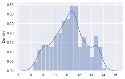
df['boxcox'].skew()
-0.008734097133920404
df['boxcox'].kurtosis()
-0.6502935539475279
Box-cox gives good results and can be used for 'charges' as Log-transformation
BMI Distribution
sns.distplot(df['bmi'])
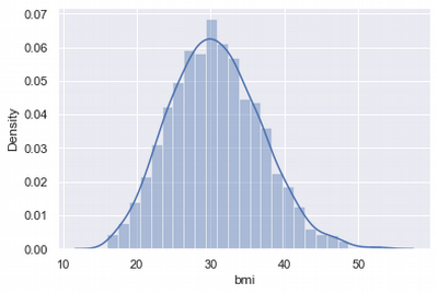
At first glance, the distribution looks normal.
Shapiro Normality test
There is one more test allows to check normality of distribution. It is Shapiro test. For this spicy library can be use
from scipy import stats
p_value = stats.shapiro(df['bmi'])[0]
if p_value <=0.05:
    print("Distribution is non-normal")
else:
    print('Distribution is normal')
Distribution is normal
df.agg(['skew', 'kurtosis'])['bmi'].transpose()
skew 0.284047 kurtosis -0.050732 Name: bmi, dtype: float64
Interim conclusions: BMI index distributed normally
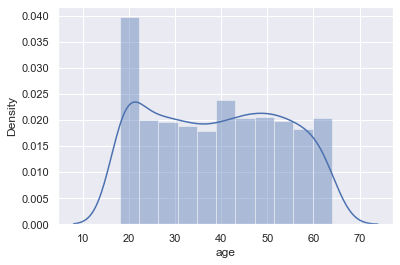
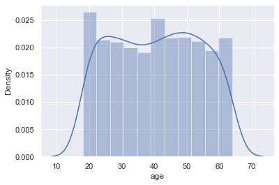
Age Distribution
As we see on the plot, ages density is quite equal, except age near 20. Let's take a look deeper
sns.distplot(df['age'])
Outliers for Age
sns.boxplot(x=df['age'])
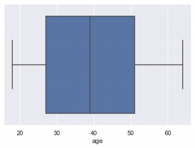
df.agg(['skew', 'kurtosis'])['age'].transpose()
skew 0.055673 kurtosis -1.245088 Name: age, dtype: float64
df.describe()['age']

count    1338.000000
mean       39.207025
std        14.049960
min        18.000000
25%        27.000000
50%        39.000000
75%        51.000000
max        64.000000
Name: age, dtype: float64
df.describe()
| age | bmi | children | charges | charges_Sqrt | charges_log | |
|---|---|---|---|---|---|---|
| count | 1338.000000 | 1338.000000 | 1338.000000 | 1338.000000 | 1338.000000 | 1338.000000 |
| mean | 39.207025 | 30.663397 | 1.094918 | 13270.422265 | 104.833605 | 9.098659 |
| std | 14.049960 | 6.098187 | 1.205493 | 12110.011237 | 47.770734 | 0.919527 |
| min | 18.000000 | 15.960000 | 0.000000 | 1121.873900 | 33.494386 | 7.022756 |
| 25% | 27.000000 | 26.296250 | 0.000000 | 4740.287150 | 68.849739 | 8.463853 |
| 50% | 39.000000 | 30.400000 | 1.000000 | 9382.033000 | 96.860893 | 9.146552 |
| 75% | 51.000000 | 34.693750 | 2.000000 | 16639.912515 | 128.995729 | 9.719558 |
| max | 64.000000 | 53.130000 | 5.000000 | 63770.428010 | 252.528074 | 11.063045 |
#samples with modified outliers
#calculate limits
feature = 'age'
x,y = boundary_values(feature)

Lower limit of age distribution: -9.0
Upper limit of age distribution: 87.0
So we see that there are no outliers in this distribution. Let's look at the "left side" counts by ages:
df.groupby(['age'])['age'].count().head(10)

age
18    69
19    68
20    29
21    28
22    28
23    28
24    28
25    28
26    28
27    28
Name: age, dtype: int64
As we see from the histogram and last output that it is near 2 times more data near 20 years, and it should be corrected. I want to find median value count for age and decrease diapasons of 18-19 years old till this median.
n = int(df['age'].value_counts().median())
df1 = df.copy()

df_19 = df1[(df1['age']==19)]
df_18 = df1[(df1['age']==18)]
df_19.describe()
df_18.iloc[n:df_18.size,:].index
df_19.iloc[n:df_19.size,:].index
df = df.drop(df_18.iloc[n:df_18.size,:].index)
df = df.drop(df_19.iloc[n:df_19.size,:].index)
df.describe()['age']

count    1255.000000
mean       40.576892
std        13.422954
min        18.000000
25%        29.000000
50%        41.000000
75%        52.000000
max        64.000000
Name: age, dtype: float64
sns.distplot(df['age'])
df.agg(['skew', 'kurtosis'])['age'].transpose()

skew        0.004377
kurtosis   -1.195052
Name: age, dtype: float64
We have reduced skewness and kurtosis a little bit.
Interim conclusions: It make sense here to leave this distribution as it is because it shows all ages more-less equally and doesn't need to be more normal distributed.
Conclusions
- In this article I described the most typical, often used and effective transformation approaches to get normal distribution. This transformations are important for the further modelling applying. Some model are sensitive for the data view and data scientist has to investigate more in a data preparation.
- As a result we can see, that Log-transformation is the most universal and effective technique. It solves most of the skewness and kurtosis problems. Box-Cox transformations are also effective and flexible.
- It can happen that data looks non-normal, but in the same time it doesn't have some outliers or very high kurtosis. In this situation it make sense to analyse such data locally and adjust it manually, for example deleting data or replacing it for a median/mean/max/min/random etc. values.